Dijkstra's Algorithm in Swift
Dejan Agostini

Last week we've talked about edge weighted digraphs in swift. This week we'll talk about a famous algorithm that's using that data structure. Dijkstra's algorithm is a simple and well-known algorithm for finding a shortest path between two points on a graph. In this article we'll implement Dijkstra's algorithm in swift and we'll implement a simple priority queue that we'll use in the algorithm. I'll assume you've read the article on edge weighted digraphs in swift. If you haven't, you might want to read that one first. It will help you understand Dijkstra's algorithm a lot better.
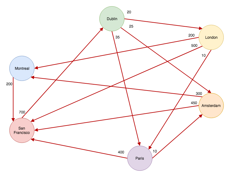 We'll use the same example with airports to discover the cheapest routes from a selected city. For example, the cheapest flight from Dublin to Paris is actually via London. Before we start implementing the actual algorithm, we'll need two things. A priority queue and an object to hold our destinations. Let's start with the priority queue first.
Quick Refresher
A graph consists of vertices which are connected by edges. Edges have a source, a destination and a weight. Last week we've implemented an edge weighted digraph that looked like this: We'll use the same example with airports to discover the cheapest routes from a selected city. For example, the cheapest flight from Dublin to Paris is actually via London. Before we start implementing the actual algorithm, we'll need two things. A priority queue and an object to hold our destinations. Let's start with the priority queue first.
Priority Queue
A priority queue is a simple data structure. Each element you add to the queue has a priority associated with it. When you dequeue an element you will always get an element with the lowest priority (or highest, depending on your implementation). We'll be implementing a minimum priority queue. Which means that the elements will be sorted from the lowest weight to the highest. To keep things as simple as possible we'll be using an array to store our queue elements. A heap would be the preferred way of storing the elements, but that goes beyond the scope of this article. In order to make our priority queue implementation as simple as possible to use, we'll use an inner class to store the data:private class QueueItem<Element: Equatable>: Comparable {
let value: Element
var priority: Double
init(_ value: Element, priority: Double) {
self.value = value
self.priority = priority
}
static func < (lhs: QueueItem<Element>, rhs: QueueItem<Element>) -> Bool {
return lhs.priority < rhs.priority
}
static func == (lhs: QueueItem<Element>, rhs: QueueItem<Element>) -> Bool {
return lhs.priority == rhs.priority
}
}
As you can see, this is a very simple generic class that only stores two properties; the priority and the actual object. It also implements the comparable interface.
Here's the implementation of the actual priority queue:
public class SimplePriorityQueue<Element: Equatable> {

    //private class QueueItem<Element: Equatable>: Comparable {//..Redacted for clarity..//}

    private var items: [QueueItem<Element>] = []

    public var isEmpty: Bool {
        return items.isEmpty
    }

    public func contains(_ item: Element) -> Bool {
        return items.contains { $0.value == item }
    }

    public func insert(_ item: Element, priority: Double) {
        if contains(item) {
            update(item, priority: priority)
        } else {
            let newItem = QueueItem<Element>(item, priority: priority)
            items.append(newItem)
            sortItems()
        }
    }

    public func update(_ item: Element, priority: Double) {
        if let existingItem = items.filter({ $0.value == item }).first {
            existingItem.priority = priority
            sortItems()
        }
    }

    public func deleteMin() -> Element? {
        guard isEmpty == false else {
            return nil
        }

        let item = items.removeFirst()
        return item.value
    }

    private func sortItems() {
        items = items.sorted(by: < )
    }
}
It's a very simple class that will sort elements based on priority after every insert or update. It has some utility methods as well but the most important ones are 'insert' and 'deleteMin'. 'deleteMin' function will return the element with the lowest priority and delete it from the queue.
Destination
Our implementation of Dijkstra's algorithm will have an array of destinations. When we initialise the algorithm class we'll provide it with a source vertex. The array of destinations will contain all the vertices on the graph. We'll use this array to calculate the cheapest route. More on that later on. The 'Destination' class is very simple:class Destination<Element: Equatable> {
let vertex: Vertex<Element>
var previousVertex: Vertex<Element>?
var totalWeight: Double = Double.greatestFiniteMagnitude
init(_ vertex: Vertex<Element>) {
self.vertex = vertex
}
}
We're initialising the class with a default value of 'Double.greatestFiniteMagnitude' for the 'totalWeight' variable. You'll see why when we go over the algorithm. The class also contains a pointer to a previous vertex on the path. We'll use this to construct a path from a source to the destination.
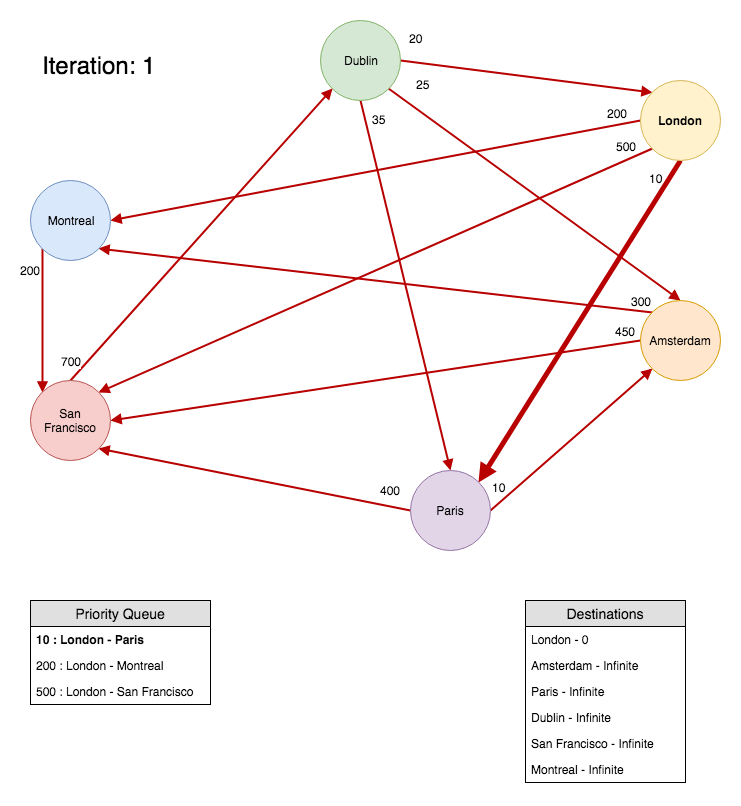 Remember, the edge has a source, a destination and a weight. But our 'Destination' object has a vertex, a previous vertex and a total weight. We'll clear this up in the next iteration example. But for now, if you look at the diagram above, you can see the priority queue has 'Paris' at the top. And as soon as it removes that vertex from the queue it will update the array of destinations (for the 'Paris' destination object) with the value of '10' and it will take the edge's source vertex and set it as a previous vertex for that 'Destination' object (in this case the source will be 'London'). The algorithm will also insert all the adjacent edges from the 'Paris' vertex into the priority queue.
Let's skip iteration 2 and see how the third iteration looks like:
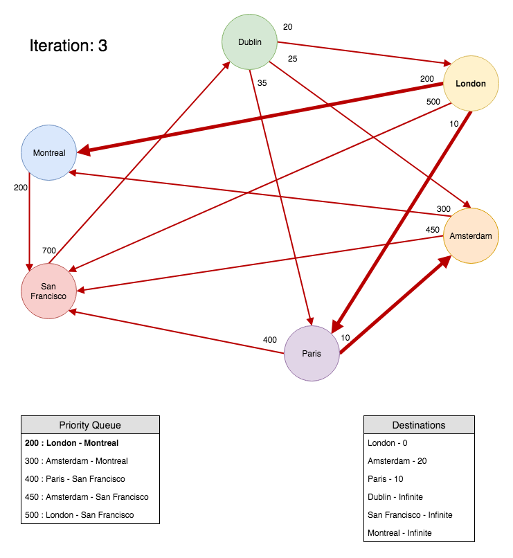 During iteration 3 we have calculated the cost to 'Amsterdam' and 'Paris'. The next cheapest edge in our priority queue is the edge that connects 'London' and 'Montreal' so we observe that edge. We remove that edge from the priority queue, add all the outgoing edges from 'Montreal' to the priority queue, because the cost to 'Montreal' is infinite, and update the destination to 'Montreal' in the destinations array.
We're going to run the algorithm in a loop until the priority queue is empty. When the algorithm is finished we'll end up with a graph that looks like this:
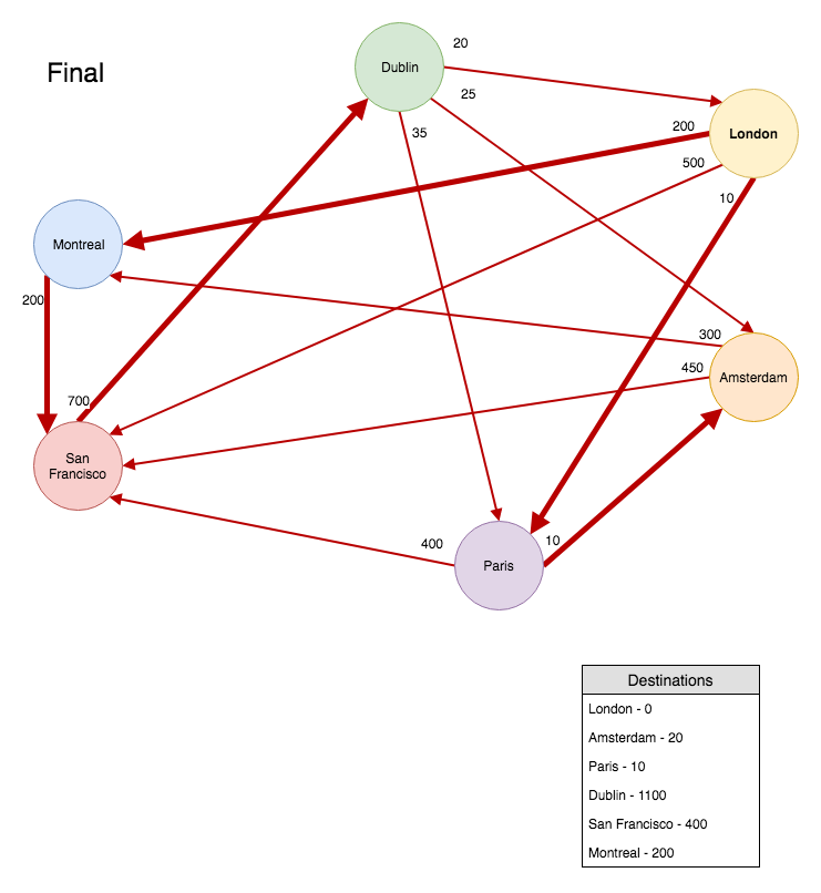 Our priority queue is empty and we have calculated the costs to all the destinations on the graph. We can see from the graph that going to 'San Francisco' would be cheaper via 'Montreal'. So the 'San Francisco' destination will have 'Montreal' set as its previous vertex.
Dijkstra's Algorithm
Now that we have the supporting classes out of the way, let's focus on the actual algorithm. We'll cover the implementation later. Dijkstra's algorithm will calculate the shortest (or cheapest) path from the source to all reachable destinations. It's using a priority queue and a list of destinations to achieve this. The algorithm starts with the source vertex. It takes all the 'outgoing' edges and adds them to the priority queue. It will take the 'cheapest' edge from the priority queue, jump to its destination and do it all over again. Let's see some pictures :) We start the algorithm with 'London' as the source vertex. Before the algorithm starts we create 'Destination' objects out of all vertices on the graph with an infinite weight (or cost) and no link to a previous vertex in the path. Because we don't know if all vertices are reachable from the selected source. In the first iteration of the algorithm we'll push the 'London' vertex onto a priority queue with a total weight of 0, since it's our source. We'll go over all the adjacent edges. Combine the edge's weight and the total weight for the current vertex and see if it's cheaper than the route we already have saved in the destinations array. In other words, we'll check if we have found a cheaper route to a destination. If we have found a cheaper route, we'll update the destinations array and insert the new destination vertex with the new priority into the queue. This is illustrated on the diagram below: Remember, the edge has a source, a destination and a weight. But our 'Destination' object has a vertex, a previous vertex and a total weight. We'll clear this up in the next iteration example. But for now, if you look at the diagram above, you can see the priority queue has 'Paris' at the top. And as soon as it removes that vertex from the queue it will update the array of destinations (for the 'Paris' destination object) with the value of '10' and it will take the edge's source vertex and set it as a previous vertex for that 'Destination' object (in this case the source will be 'London'). The algorithm will also insert all the adjacent edges from the 'Paris' vertex into the priority queue.
Let's skip iteration 2 and see how the third iteration looks like:
 During iteration 3 we have calculated the cost to 'Amsterdam' and 'Paris'. The next cheapest edge in our priority queue is the edge that connects 'London' and 'Montreal' so we observe that edge. We remove that edge from the priority queue, add all the outgoing edges from 'Montreal' to the priority queue, because the cost to 'Montreal' is infinite, and update the destination to 'Montreal' in the destinations array.
We're going to run the algorithm in a loop until the priority queue is empty. When the algorithm is finished we'll end up with a graph that looks like this:
 Our priority queue is empty and we have calculated the costs to all the destinations on the graph. We can see from the graph that going to 'San Francisco' would be cheaper via 'Montreal'. So the 'San Francisco' destination will have 'Montreal' set as its previous vertex.
In A Few Simple Steps
Just remember these few steps:- Check all the outgoing edges of a vertex
- If the route you're checking is cheaper than the one you have saved in the 'Destinations' array, do step 3.
- Update the 'Destinations' array with the new cheapest route and insert the destination into the priority queue
Implementation
After all that theory and preparation it's time to actually implement the algorithm. Our class will have two instance variables. One for the priority queue and another for the destinations. In the initialiser we'll fill out the destinations array with all the vertices from the graph and set the total weight of them to be infinite. The last thing we'll do in the initialiser is to insert the source vertex into the priority queue and keep calling the 'relax' function until the queue is empty:private var destinations: [Destination<Element>] = [] // Dictionary would be more efficient. Using array for simplicity.
private var priorityQueue: SimplePriorityQueue<Vertex<Element>> = SimplePriorityQueue<Vertex<Element>>()
init(_ graph: EdgeWeightedDigraph<Element>, source: Vertex<Element>) {
graph.vertices.forEach { self.destinations.append(Destination($0)) }
let sourceDestination = destination(for: source)
sourceDestination.totalWeight = 0.0
priorityQueue.insert(source, priority: 0.0)
while (priorityQueue.isEmpty == false) {
if let min = priorityQueue.deleteMin() {
relax(min)
}
}
}
Remember those three steps from above. They're all performed in the 'relax' function:
private func relax(_ vertex: Vertex<Element>) {
	vertex.adjacentEdges.forEach { (edge) in

		let edgeDestination = edge.destination
		let nextDestination = destination(for: edgeDestination)
		let currentDestination = destination(for: vertex)

		if nextDestination.totalWeight > (currentDestination.totalWeight + edge.weight) {
			nextDestination.totalWeight = currentDestination.totalWeight + edge.weight
			nextDestination.previousVertex = edge.source

			priorityQueue.insert(nextDestination.vertex, priority: nextDestination.totalWeight)
		}
	}
}
For every adjacent edge in the vertex we get the next destination from the array of destinations. We then check to see if the existing total weight of the next destination is more expensive than the combined weights of the current destination and the edge weight for the next destination. What this means is, we're looking to see if we have a cheaper route, nothing more. If the current edge is giving us a cheaper route then we'll update the array of destinations with the new total weight and set the previous vertex to be the source vertex of the edge. We'll call this function in a loop until our priority queue is empty. When the function completes we'll have an array with shortest paths to all reachable destinations.
We have a couple of utility functions in our class that we won't go over. We'll only talk about the function that we use to get the shortest path:
public func pathTo(_ vertex: Vertex<Element>) -> [Vertex<Element>]? {
	guard hasPathTo(vertex) else {
		return nil
	}

	var results: [Vertex<Element>] = [vertex]

	var currentDestination = destination(for: vertex)
	while let previousVertex = currentDestination.previousVertex {
		results.insert(previousVertex, at: 0)
		currentDestination = destination(for: previousVertex)
	}

	return results
}
First we check if we have a path to the passed in vertex. We simply check the destinations array and see if the cost to that destination is not infinite. If we have the path to the vertex, we fetch the destination object for that vertex and start building a path from the destination back to the source.
Test It Out
We already created our graph last week, so we'll just use that. At the end fo that function you can create our new Dijkstra's algorithm and print the shortest path between 'London' and 'Dublin':let dijkstra = DijkstraShortestPath(graph, source: london)
print("Path to Dublin: ", dijkstra.pathTo(dublin))
Our example output will look like this:
Path to Dublin:  Optional([
[Vertex]: London | [Adjacent Edges]: [[
[Edge] [Destination]: Paris - [Weight]: 10.0,
[Edge] [Destination]: Montreal - [Weight]: 200.0,
[Edge] [Destination]: San Francisco - [Weight]: 500.0]],
[Vertex]: Montreal | [Adjacent Edges]: [[
[Edge] [Destination]: San Francisco - [Weight]: 200.0]],
[Vertex]: San Francisco | [Adjacent Edges]: [[
[Edge] [Destination]: Dublin - [Weight]: 700.0]],
[Vertex]: Dublin | [Adjacent Edges]: [[
[Edge] [Destination]: London - [Weight]: 20.0,
[Edge] [Destination]: Amsterdam - [Weight]: 25.0,
[Edge] [Destination]: Paris - [Weight]: 35.0]]])
In this test we set 'London' as our source, but you can set any vertex on the graph to be the source. From the test that we just ran, we can see that the cheapest route from 'London' to 'Dublin' i via 'Montreal' and 'San Francisco'.